Downsample Data

Downsampling EEG data during FPVS preprocessing.

Why use a lower sampling rate?

The sampling rate tells us how many readings each channel contributes per second. A recording collected at 1,000 Hz contains 1,000 voltage readings per channel every second. That detail is useful, but it also makes the data matrix larger.

Downsampling creates an analysis copy with fewer time samples. It can save memory and disk space, as explained in EEGLAB’s resampling guide. Fewer samples can also speed processing when high frequencies or very precise timing are unnecessary; MNE’s guide explains the trade-off. This is optional: choose a rate that preserves your analysis, and keep the original raw recording.

Fewer columns, the same recording

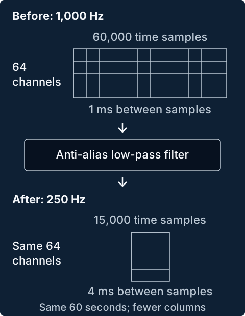
Return to the matrix from Import Raw Data: rows are channels, columns are time samples, and each cell contains a voltage reading. Downsampling reduces the number of columns while keeping the same channels and recording duration.

For a 60-second recording with 64 EEG channels:

• At 1,000 Hz: 64 rows × 60,000 columns = 3,840,000 readings, spaced 1 millisecond apart.
• At 250 Hz: 64 rows × 15,000 columns = 960,000 readings, spaced 4 milliseconds apart.

This example has one quarter as many readings. If the numerical storage type stays the same, the voltage array uses about one quarter of the space; the whole file’s size also depends on metadata and compression. The voltage unit stays the same—downsampling does not mean dividing microvolt values by four.

Downsampling reduces the time columns while retaining the channel rows. This 1,000-to-250 Hz example includes an anti-alias filter before the reduction. Only a few illustrative cells are drawn.

Filter before removing samples

For a simple four-fold reduction, the basic idea is to apply an appropriate low-pass filter along the time dimension of each EEG channel, then retain every fourth sample of the filtered signal. The filter reduces fast fluctuations that the new sampling rate cannot represent. This filter-then-reduce procedure is described in SciPy’s decimation documentation.

Without that filter, higher-frequency activity can appear falsely at lower frequencies—a problem called aliasing. Deleting three out of every four columns of the raw matrix is therefore not a safe substitute for a proper resampling operation. EEGLAB’s resampling function includes anti-alias filtering. Other rate changes may calculate new samples rather than simply select existing ones; SciPy’s polyphase resampling guide gives an example.

This filtering happens as part of downsampling, even though the separate frequency-filtering step comes later in this workflow. Filtering after an unprotected reduction cannot undo aliasing that has already occurred.

Choose a rate for the analysis

The theoretical upper frequency limit is half the sampling rate, called the Nyquist frequency. At 250 Hz, that limit is 125 Hz. In practice, keep the frequencies of interest comfortably below it and allow room for the anti-alias filter’s transition band. MNE’s resampling guidance discusses this relationship. The 250 Hz example above is an illustration, not a recommended rate for every dataset.

For FPVS, consider the highest base or oddball harmonic you plan to analyse, rather than only the stimulation frequency. If a 6 Hz base response is assessed through its tenth harmonic, the signal of interest extends to 60 Hz. The new rate and filter must preserve that range. Once downsampling removes higher-frequency information, increasing the sampling rate later cannot recover it.

Timing also becomes coarser: in our example, the sample grid changes from 1 to 4 milliseconds. Update the sampling-rate metadata and any event sample indices together; indices from the original recording cannot be reused unchanged. MNE’s event-timing guidance explains the timing implications and the option to resample continuous data and its event array together. Check that event counts and times still match the experiment before continuing.